JEL codes: C14; C99; E31
Códigos JEL: C14; C99; E31
RESUMEN
En esta investigación, exponemos la capacidad de las pruebas de Kolmogórov-Smirnov de dos muestras para estudiar la existencia de efectos asimétricos (una innovación metodológica) y las dinámicas de experimentos naturales. Para mostrar ambas aplicaciones, analizamos la inflación latinoamericana desde 2020 hasta 2022: comprobamos que la instauración de políticas de cierres de comercios (debidas a la pandemia del covid-19) fue menos deflacionaria de lo inflacionaria que fue su eliminación; y comprobamos que, en general, la inflación latinoamericana en nuestro periodo de estudio obedece a factores idiosincráticos más allá de la política monetaria de los Estados Unidos.
1. INTRODUCTION
In macroeconomics, formally verifying causality is always a worthy challenge, but usually an unsatisfactory one. Henschen (2018) postulates that macroeconometrics has four notions of causality: Granger causality (predictive ability of lags of one variable on another variable); Hendry causality (super-exogeneity); Hoover causality (privileged parameterization); and Angrist and Kuersteiner causality (potential outcome paradigm applied to monetary policy). But either way, the end is the same: the feeling of speaking in very different terms than microeconometrics. Feeling disheartened by these circumstances can hardly be condemned as an inferiority complex; those elegant constructions of counterfactuals and control groups from comparable agents feel like the closest economics can get to laboratory experiments without losing external validity.
The two sample Kolmogorov-Smirnov test somewhat brings us closer to that dialect. Macroeconomics has used it specially to evaluate structural changes. The tactic is as follows: 1) there is an apparently distortive event, and we want to evaluate its effects on a particular time series; 2) we divide the series in two parts (before and after the event); and 3) the K-S test evaluates the hypothesis that both parts belong to the same distribution.
But we must be honest. For example, saying that the entry and exit of the world pandemic crisis of our decade had deflationary and inflationary effects, respectively, is a truism. However, this statistical test has much greater capabilities. In fact, in natural sciences, its traditional use is precisely within the laboratory: to compare treatments and controls.
With that inspiration, in this paper we show how useful the two-sample K-S tests can be for evaluating natural experiments. Specifically, we will put under scrutiny the theory that Latin American inflation since the recovery from the COVID-19 global crisis has been imported from the monetary policy of the Federal Reserve of the United States (see section 3.3).
We also present what, at least to the author’s knowledge, constitutes a methodological innovation: the use of K-S tests to diagnose asymmetric effects. In that spirit, we will evaluate whether the establishment of pandemic restrictions caused deflation to a lesser extent than the inflation caused by their lifting — again, focusing on the Latin American experience.
Now, before moving on with the rest of the paper, we must issue a warning: our preference for the Kolmogorov-Smirnov test is solely due to its popularity. All the virtues of this tool for the present work are shared by any non-parametric test that attacks the so-called «two-sample problem»; and there is no doubt that, in the catalog of such tests, there may be better ones than the Kolmogorov-Smirnov test depending on the circumstances.
The paper is organized as follows: in section 2 we review the works that precede ours in methodological (double-sample K-S tests applied in economics) and thematic (inflation since 2020) terms; in section 3 we detail our databases and empirical strategy; section 4 presents and interprets our results; and in section 5 we make a brief synthesis as a conclusion.
2. LITERATURE REVIEW
In the methodological department, our most abundant precedents are those that take advantage of the traditional way macroeconomics use K-S tests: to check if an event establishes a before and after in a series. There are works such as Reinhart and Reinhart (2010), where long-term trend changes in real GDP, unemployment, inflation, credit, and real estate prices are studied for 60 countries before and after international shocks following World War II. In another example, Mian, Sufi, and Trebbi (2014) use K-S tests in 70 countries to verify the increase in legislative party fragmentation that occurs after a financial crisis —as a reason why debt relief reforms that could alleviate downturns are not approved. Ngure and Waititu (2021) also develop the test in a reverse procedure: a statistic that indicates the disruption date for the exchange rate series between the US dollar and the Kenyan shilling.
However, as we anticipated in the introduction, the home of K-S tests outside of the social sciences is the laboratory. Therefore, it should not surprise us that experimental economics has taken advantage of its benefits: Holt and Laury (2005) evaluate whether participating in a low-stakes payment decision before participating in a high-stakes payment decision disrupts risk aversion. In general, Goerg and Kaiser (2009) can be consulted for a record of non-parametric tests that address «the two-sample problem» applied in experimental economics.
Now, in the thematic department, our precedents are the works aimed to understand inflation fluctuations between 2020 and 2022. Abdelkafi, Loukil, and Romdhane (2022) make generalized method- of-moments estimates on the influence that COVID-19 infections and government measures (public awareness and subsidies, specifically) exert on inflation and the exchange rate in selected Latin America and Asia economies.
Moving on to the recovery period, Jordà, Liu, Nechio, and Rivera-Reyes (2022) argue, by estimating a Phillips curve, that the stimulation of disposable income from fiscal aid was what caused US inflation to outpace that of other Organization for Economic Co-operation and Development (OECD) nations. Also estimating a Phillips curve in the United States, Ball, Leigh, and Mishra (2022) find that the increase in underlying inflation since 2021 is explained mainly by: 1) pressure on the labor market in terms of more job openings relative to unemployment; and 2) the transfer of very persistent non-underlying inflation shocks.
A secondary thematic axis of our work is the asymmetric responses of inflation to the same stimulus. The stimulus that has aroused the interest of researchers the most has been monetary policy. See Santoro, Petrella, Pfajfar, and Gaffeo (2014) for an extensive review of antecedents in this area; along with a behavioral model that rationalizes the regularity that they all detect: in response to monetary policy, output increases more during recessions than it decreases during expansions; inflation, on the other hand, exhibits a symmetric effect in both phases of the cycle—in section 4, we will see that this does not appear to be the case for business closure policy.
3. METHODOLOGY
3.1 Data
The main database for our study is the Economic Information System (SIE) of Fondo Latinoamericano de Reservas (FLAR). In particular, the time series for prices, which records the monthly consumer price index (CPI) for the following countries: Argentina, Bolivia, Brazil, Chile, Colombia, Costa Rica, Ecuador, El Salvador, Guatemala, Honduras, Mexico, Nicaragua, Panama, Paraguay, Peru, Dominican Republic, Uruguay, and Venezuela.
We will consider the period that goes from January 2017 because it is the first complete year for which there is data for all countries in the sample. We exclude Jamaica and Guatemala from our study because they do not have data for the second half or more of 2022; likewise, we exclude Argentina and Venezuela because of their hyperinflationary dynamics, which could contaminate the comparative analysis we pursue. Of the remaining data, only Brazil has a missing value (August 2022) between two known values; therefore, we use linear interpolation to complete the series. Finally, we choose August 2022 as the end of the period because it is the last month for which there is information for all countries.
As a measure of inflation, we will use the year-on-year log-change of the price series to eliminate the seasonality of the CPI and to ensure symmetry in increases and decreases. This is another reason to exclude hyperinflationary economies: this desirable property of natural logarithms is only valid for small growth rates (Romero, 2020). Thus, we end up with a sample of 15 Latin American nations comprising their logarithmic year-on-year inflation rates from January 2018 to August 2022.
While this is the series of primary interest in our study, we will need the real Gross Domestic Product (GDP) series of Ecuador, El Salvador, and Panama to construct a hypothetical dollarized economy (see section 3.3). Therefore, we obtained from the World Bank the annual GDP data at constant (2010) prices for these three economies for 2018, 2019, 2020, and 2021 (for 2022 we will use the 2021 data).
Finally, it should not be forgotten that the range of years that most concerns us, 2020-2022, is marked by a latent variable: the COVID-19 pandemic. To establish a less subjective criterion for designating the dates that mark the beginning of the recovery from the health crisis, we will use the COVID Stringency Index of the Oxford Coronavirus Government Response Tracker (OxCGRT). This index takes values from 0 to 100 and consists of a weighted sum of the following factors: closures of educational centers, workplaces, and public transport; cancellation of public events; restriction on meetings, movement within the country, and international travel; orders to stay at home; and information campaigns.
3.2. Kolmogorov-Smirnov tests
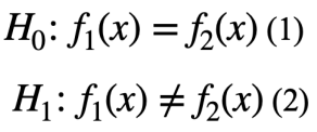
We will follow the exposition and notation of Young (1977). The setting in which K-S tests are applied is one in which we have two histograms 〖f_n〗_1 (x) and 〖f_n〗_2 (x) of n_1 and n_2observations, respectively. It is assumed that these histograms are samples from two continuous probability density functions: f_1 (x) and f_2 (x), in that order. The two-sample Kolmogorov-Smirnov test has the following null hypothesis (H_0) and alternative hypothesis (H_1):
To test them, the sample probability distribution functions are constructed from the histograms as follows:
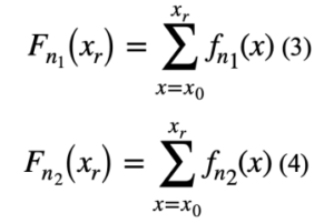
where x_r is the horizontal value of the r-th division of the histogram.
With this information, the test statistic is constructed:
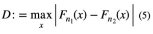
There are two key details. First: as can be seen, the statistic is the maximum distance that the sample probability distribution functions have between each other. Intuitively, this can be thought of as the most important point; because outside of it, the distributions, by definition, are more similar. Second: the test is non-parametric and as such, we do not assume a particular distribution for the two samples involved; to understand how to obtain the p-value and the critical values in the test, Hodges (1958) can be consulted as a classic reference; or Facchinetti (2009) for a modern method that reduces the problem to a linear system. In either case, the prominence of binomial counting arguments is noticeable.
3.3. Empirical strategy
Lizano (2022) informally hypothesized about the inflation take-off in Costa Rica that occurred since the recovery from the COVID-19 pandemic. His conjecture was that this inflation was imported from the United States; specifically, that it was the result of an aggressive monetary policy by the Federal Reserve and, secondarily, the paralysis of supply chains that the US recovery had inflicted. We will test this hypothesis, not only for Costa Rica but for all Latin America. To do so, we will design a natural experiment.
We will create the inflation series of an artificial economy; a ‘dollar basket’. We will take the inflation series of Ecuador, El Salvador, and Panama and calculate their weighted average, using the real GDP of the respective year as the weight. The reason for proceeding as we did is that these are three dollarized nations : that is, our ‘dollar basket’ has the characteristics of a Latin American economy, but all shocks to its local currency are the same shocks that the US dollar receives. Our artificial economy is productively Latin America and monetarily the United States.
What we will do with the other 12 inflation series is to compare them one by one, from January 2021 to the end of our series (August 2022), with the dollar basket series using a K-S test. Thus, if the null hypothesis that they come from the same distribution is not rejected, it means that during the study period, the inflation of the respective country is caused by US monetary policy shocks. Otherwise, it follows that there are idiosyncratic factors that make it impossible to categorize inflation as 100% imported from the United States.
In another section, as we hinted in the introduction, we want to present a novel applicability of K-S tests: the evaluation of asymmetric effects. We want to find out if the deflationary effect that the COVID-19 crisis had was greater than the inflationary effect that the recovery from it had. To define the start of the pandemic and the recovery, we need an objective way to locate their dates. For the first date, it is straightforward: March 2020. For the second date, although not a perfect decision, it is defensible: we will use as a proxy, for each country, the first month after the COVID Stringency Index reached its 2021 maximum.
Provided with our definitions, we will do the following:
Step 1: We will perform K-S tests for our 15 countries, comparing the segment of the inflation series that goes from January 2019 to March 2020, with the segment of the inflation series that goes from April 2020 to the month before the respective country’s recovery.
Step 2: We will perform K-S tests for our 15 countries, comparing the segment of the inflation series that goes from April 2020 to the month before the respective country’s recovery, with the segment of the inflation series that goes from the month of the respective country’s recovery to the end of the series.
Step 3: The p-values associated with Step 1 are a (inversely proportional) measure of the alterations that the COVID-19 pandemic caused in the inflation distribution; the p-values associated with Step 2 are a measure (inversely proportional) of the alterations that the pandemic recovery caused in the inflation distribution. Thus, if we find a regularity when comparing both sets of p-values (that those from Step 1 are systematically higher than those from Step 2, or vice versa), it will tell us what caused a greater impact on inflation: the onset or the end of the health crisis, rigorously, the appearance or disappearance of the restrictions associated with it.
Finally, as a general comment for our entire methodology, we should note that we will use the exact p-value rather than the asymptotic one to evaluate our hypotheses. This is because the latter is very sensitive to sample size; particularly, it excessively fails to reject the null hypothesis as the number of observations decreases.
4. RESULTS
In Table 1, we present our results regarding the experiment that compares each economy to the ‘dollar basket’.
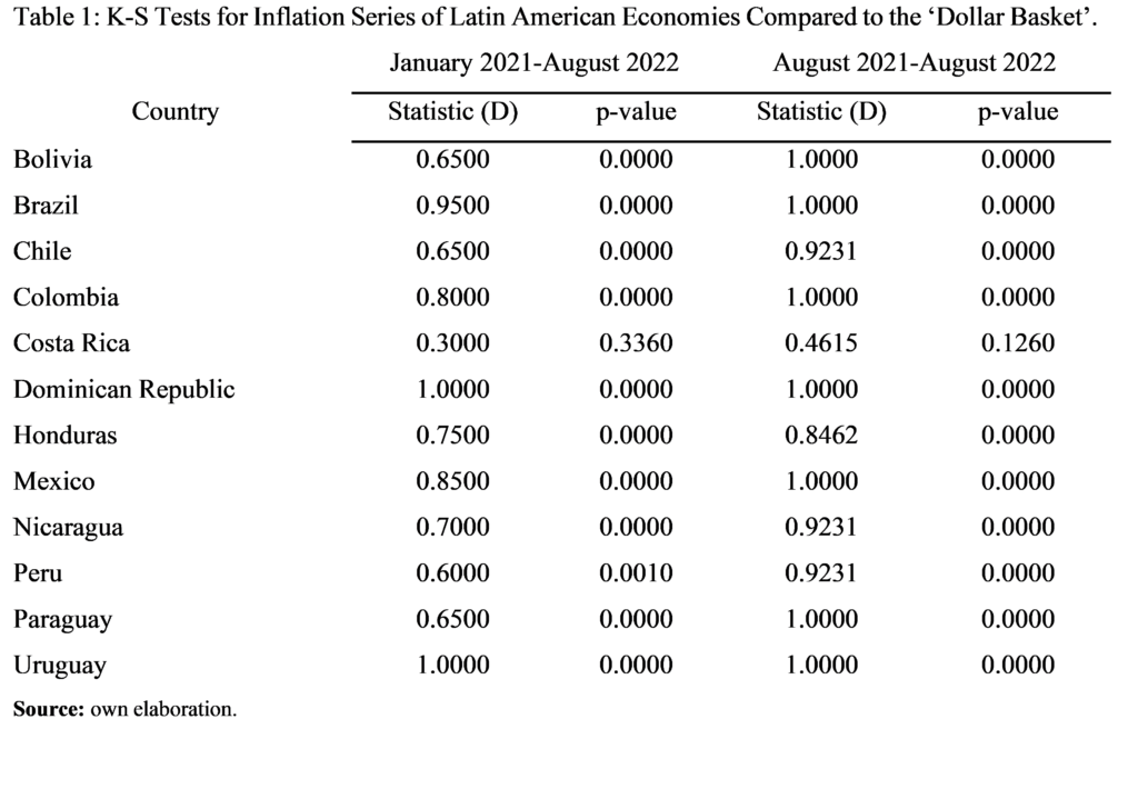
As can be seen, for robustness purposes, we not only tested our hypothesis using the start date of the US recovery (under our criterion with the COVID Stringency Index): January 2021. We also used the date from which all Latin American economies had already started their recovery (again, under our criterion with the COVID Stringency Index): August 2021. And the results are the same: 1) for Costa Rica, it cannot be rejected, at any conventional significance level, that the distribution of its inflationary process is different from that of our hypothetical economy; and 2) for the rest of the sample, this hypothesis is rejected, at all conventional significance levels— see Ulate (2021) for a modeling of the weakness of US monetary policy when operating in the zero lower bound area.
Of course, our results do not indicate that US monetary policy is irrelevant to the rest of the inflationary processes in Latin America. Rather, it indicates that a set of idiosyncratic factors must be added to the explanation. For example, Carrera and Ramirez (2020) find that the inflation of Chile, Mexico, Peru, and Colombia has been insensitive to the measures of quantitative easing implemented by the Federal Reserve. However, as reviewed by de Paula, Saravia, and Ferreira (2022), these countries implemented their own unconventional monetary policy tools.
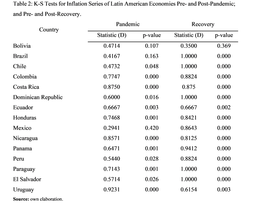
For the asymmetric effects of sanitary restrictions, we report our results in Table 2. As can be seen, p-values are systematically lower for the K-S test associated with economic recovery. This represents evidence that the rehabilitation of economic activity caused stronger inflationary shocks than the deflationary shocks caused by the depression.
We theorize that this asymmetry is due to the following dynamic: when health restrictions were applied, the result was a large exogenous contraction of aggregate demand to which aggregate supply responded endogenously. On the other hand, when the restrictions were lifted, not only did aggregate demand expand exogenously (aided by the recovery itself, but also by variations in disposable income introduced to alleviate the crisis) but it also forced production to a level above the capacity with which it was left by the crisis.
We can think of a situation like the one described in Figure 1: first, the demand curve shifts backwards (D_1), but during the time it takes to return to its original position (D_0), a latent supply curve (S_1) is activated: more inelastic than the original (S_0) because it has become accustomed to the lower input requirement and lower selling capacity in specific sectors.
Figure 1: aggregate supply beginning a regime of lower production.
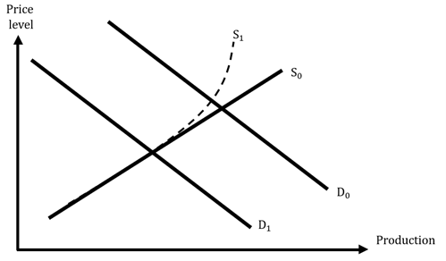
Source: own elaboration.
Empirical support for this theory can be found in Shapiro (2022): through a disaggregated analysis of the data, he identifies which goods experience price and quantity movements in the same direction, and which move in the opposite direction. As a result, he concludes that 50% of post-COVID-19 US inflation is due to supply factors, 33% to demand factors, and the rest to unidentified factors. Bringing up this case has a purpose: it helps us to understand that the process described above, in a context of sudden excess capacity changes, affects both large and small economies; and this fact gives rise to what has colloquially been called the global «bottleneck» problem. Thus, re-inflation has an international force that also helps to explain why it was more powerful than pandemic deflation: the asymmetrical effects found in 13 of our 15 countries.
It remains to explain the exceptions: Bolivia and Uruguay. The Bolivian case can be understood because the prices that have experienced the greatest increase worldwide, namely food and fuel, are regulated/subsidized in Bolivia (Olmo, 2022). The Uruguayan case, on the other hand, we suggest is due to the abnormally positive performance in terms of the COVID Stringency Index: (apart from March 2020) the only spike occurs just before the month of recovery, so it is understandable that the lifting of internal restrictions was not as influential. Both phenomena may point to limitations of our study: Bolivia because the CPI is an imperfect quantifier of inflation; and Uruguay because the way we defined recovery is also imperfect for its purpose.
As another limitation, and since we have discussed the existence of relevant international shocks, it could be argued that our asymmetrical effects are not entirely explained by returning to normality; that the Russian-Ukrainian war is also responsible. And whoever argues this might be right. But everything seems to indicate that the war has played a secondary role: for the 12 countries for which we found asymmetrical effects to three decimal places of significance, we conducted K-S tests comparing inflation from the month of recovery until February 2022 (the month of the Russian invasion) with inflation until the end of the series; only for a third of them does the test reject the null hypothesis at three decimal places of significance (Honduras, Nicaragua, El Salvador, and Paraguay); and they all have in common that oil is their largest or second-largest import (Observatory of Economic Complexity, 2021).
5. CONCLUSIONS
We found that there were asymmetric effects of business closure policies, aimed at preventing the COVID-19 pandemic, on the inflation of Latin American economies. Specifically, the implementation of these regulations, in general, was less deflationary than their elimination was inflationary.
Additionally, for these same Latin American economies, we found that US monetary policy, in general, does not provide a complete explanation for the rise in their general prices levels. While we cannot rule out its influence, we can conclude that it had to be accompanied by idiosyncratic factors to bring Latin American inflation rates to their current state.
Finally, based on the methodology that we used to achieve these results; we presented the usefulness of the two sample Kolmogorov-Smirnov tests in two areas. Natural experiments (an area that is rarely explored but which applicability has always been tacit in the experimental economics literature; and the study of asymmetric effects) a methodological innovation, again, at least as far as the author is aware.
REFERENCES
Abdelkafi, I., Loukil, S. & Romdhane, Y. (2022). Economic uncertainty during COVID-19 pandemic in Latin America and Asia. Journal of the Knowledge Economy, 13(1) 1-20. doi:https://doi.org/10.1007/s13132-021-00889-5
Ball, L., Leigh, D. & Mishra, P. (2022, October). Understanding US Inflation During the COVID Era (National Bureau of Economic Research Working Paper No. w30613). doi:https://doi.org/10.3386/w30613
Banco Mundial (2022). DataBank [Conjunto de datos]. PIB (a precios constantes de 2010).
Recuperado de: https://datos.bancomundial.org/indicator/NY.GDP.MKTP.KD
Carrera, C. & Ramírez, N. (2020). Effects of US quantitative easing on Latin American economies. Macroeconomic Dynamics, 24(8), 1989-2011. doi:https://doi.org/10.1017/S1365100519000075
De Paula, L., Saravia, P. y Ferreira, M. (2022, January). Monetary policy in Latin America during the COVID-19 crisis: Was this time different? (Instituto de Economía, UFRJ Discussion Paper No. 02-2022). Recuperado de: https://www.ie.ufrj.br/images/IE/TDS/2022/TD_IE_002_2022_PAULA_SARAIVA_FERREIRA.pdf
Facchinetti, S. (2009). A procedure to find exact critical values of Kolmogorov-Smirnov test. Statistica Applicata–Italian Journal of Applied Statistics, 21(3-4), 337-359. Recuperado de: https://publires.unicatt.it/en/publications/a-procedure-to-find-exact-critical-values-ofkolmogorov-smirnov-te-7
Fondo Latinoamericano de Reservas (2023). Sistema de Información Económica. [Conjunto de datos]. Prices. Recuperado de: https://flar.com/sie/
Goerg, S. & Kaiser, J. (2009). Nonparametric testing of distributions—the Epps–Singleton two-sample test using the empirical characteristic function. The Stata Journal, 9(3), 454-465. doi:https://doi.org/10.1177/1536867X0900900307
Henschen, T. (2018). What is macroeconomic causality? Journal of Economic Methodology, 25(1), 1-20. doi: https://doi.org/10.1080/1350178X.2017.1407435
Hodges, J. (1958). The significance probability of the Smirnov two-sample test. Arkiv för matematik, 3(5), 469-486. doi:https://doi.org/10.1007/BF02589501
Holt, C, & Laury, S. (2005). Risk aversion and incentive effects: new data without order effects. American Economic Review, 95(3), 902-904. doi:https://doi.org/10.1257/0002828054201459
Jordà, Ò., Liu, C., Nechio, F. & Rivera-Reyes, F. (March 28th, 2022). Why Is US Inflation Higher than in Other Countries? Federal Reserve Bank of San Francisco Economic Letters. Recuperado de: https://www.frbsf.org/economic-research/publications/economic-letter/2022/march/why-is-us-inflation-higher-than-in-other-countries/
Lizano, E. (25 de febrero del 2022). La inflación ¿otra vez? El Financiero. Recuperado de: https://www.elfinancierocr.com/opinion/la-inflacion-otra-vez/26V45CPKCVCQPOMOH2Y73MJXZI/story/
Mian, A., Sufi, A., & Trebbi, F. (2014). Resolving debt overhang: Political constraints in the aftermath of financial crises. American Economic Journal: Macroeconomics, 6(2), 1-28. doi:https://doi.org/10.1257/mac.6.2.1
Ngure, J., & Waititu, A. G. (2021). Change Point Estimation in Volatility of a Time series using a Kolmogorov Smirnov Type Test Statistic. Machakos University Journal of Science and Technology, 2(3), 1-15. doi:http://ir.mksu.ac.ke/handle/123456780/12656
Observatory of Economic Complexity (2021). Datos internacionales. [Conjunto de datos]. Trade. Recuperado de:https://oec.world/es/data-availability
Olmo, G. (April 25th, 2022). Cómo se ha librado Bolivia de la inflación que recorre América Latina (y por qué no es tan buena noticia como parece). BBC News Mundo. Recuperado de:https://www.bbc.com/mundo/noticias-america-latina-61184894
Our World in Data (2022). Oxford Coronavirus Government Response Tracker. [Conjunto de datos]. COVID Stringency Index. https://ourworldindata.org/covid-stringency-index
Reinhart, C. & Reinhart, V. (2010, septiembre). After the fall (National Bureau of Economic Research Working Paper No. w16334). Recuperado de:http://www.nber.org/papers/w16334.pdf
Romero, R. (2020). Apuntes para el curso EC-4301: Macroeconometría. EC-4301: Macroeconometría. Universidad de Costa Rica.
Santoro, E., Petrella, I., Pfajfar, D. & Gaffeo, E. (2014). Loss aversion and the asymmetric transmission of monetary policy. Journal of Monetary Economics, 68(9), 19-36. doi:https://doi.org/10.1016/j.jmoneco.2014.07.009
Shapiro, A. (June 21st, 2022). How Much do Supply and Demand Drive Inflation? Federal Reserve Bank of San Francisco Economic Letters. Recuperado de:https://www.frbsf.org/economic-research/publications/economic-letter/2022/june/how-much-do-supply-and-demand-drive-inflation/#:~:text=Specifically%2C%20supply%2D%20and%20demand%2D,its%20pre%2Dpandemic%20average%20level.
Ulate, M. (2021). Going Negative at the Zero Lower Bound: The Effects of Negative Nominal Interest Rates. American Economic Review, 111(1), 1-40. doi:https://doi.org/10.1257/aer.20190848
Young, I. (1977). Proof without prejudice: use of the Kolmogorov-Smirnov test for the analysis of histograms from flow systems and other sources. Journal of Histochemistry & Cytochemistry, 25(7), 935-941. doi:https://doi.org/10.1177/25.7.894009